
Quantum GIS (QGIS) は視覚化、管理、編集、データ解析、印刷できる地図作製に使える ユーザフレンドリーなデスクトップ GIS クライアントです。
Contents
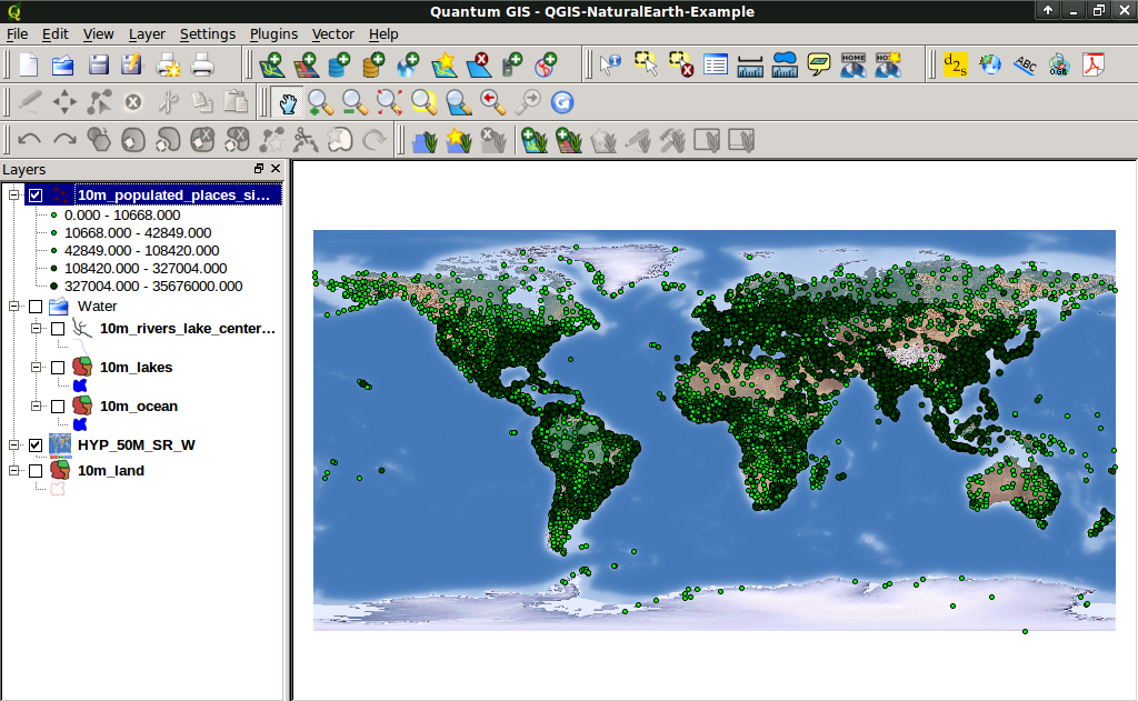
既存の QGIS プロジェクト を開き、レイヤのオンとオフを切り替えるところから始めましょう。
Geospatial ‣ Desktop GIS ‣ QGIS から QGIS を起動し、メニューバーから Project ‣ Open を選択してください。
ファイル QGIS-NaturalEarth-Example.qgs を選択し、 Open をクリックしてください。
レイヤツリーから ne_10m_populated_places を選択してください
人口の多い地域が、たくさんの緑のドットで表示されます:
Try dragging layers up and down in the legend and see how that affects visibility of the layers below.
Have a look at the tools on the tool bar. Try panning, zooming in, and zooming back out to full extent again. Find these tools next to the hand icon. If the toolbars seem cluttered you can drag them around and turn them on and off by right clicking. You can also zoom in and out with the mouse wheel, and pan with a left-click drag.
Now let’s try customising the style of the map.
Let’s now create a new QGIS project and load our own data.
Let’s now include a layer from a Postgres database.
In the layer list on the left, untick the ne_10m_admin_0_countries visibility check box to temporarily hide it.
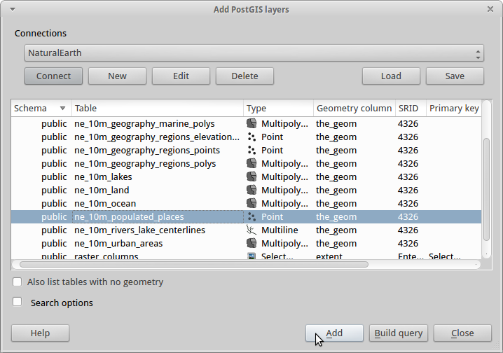
Choose Layer ‣ Add PostGIS Layers....
Select the “Natural Earth” connection and press Connect.
Select ne_10_populated_places and click Add.
Zoom in on the United States using the mouse wheel and left-click drag to navigate.
Right click on ne_10m_populated_places in the layer list to get a context menu, then select Properties.
Let’s represent one of the database attributes in the data as a bubble plot. In the middle of the Layer Properties window, drag the Transparency slider to 50%, press the Advanced button and select Size scale field, then choose elevation (it’s in about the middle of the list), and finally set the symbol Size scaling to 0.02. Then click Ok.
You can then click on the query button on the toolbar (cursor arrow with a blue “i”) and then on the map canvas bubbles to view information about the individual cities.
There have been many plugins written for QGIS which extend QGIS’s core functionality. One of the more powerful is the GRASS plugin, which taps into the hundreds of geospatial processing modules available from GRASS GIS.
Clear the slate with Project ‣ New.
Choose Plugins ‣ Manage and Install Plugins..., then scroll down or type grass into the Search box, and select the GRASS plugin.
Connect to an existing GRASS workspace with Plugins ‣ GRASS ‣ Open mapset.
Within the central GRASS data base are a number of sample datasets. We’ll load the Spearfish location, and the user1 mapset within it. Choose the spearfish60 Location and user1 working mapset, then click Ok.
To add a map to the QGIS layer list, choose Plugins ‣ GRASS ‣ Add GRASS raster layer.
In the PERMANENT mapset select the aspect map and click Ok.
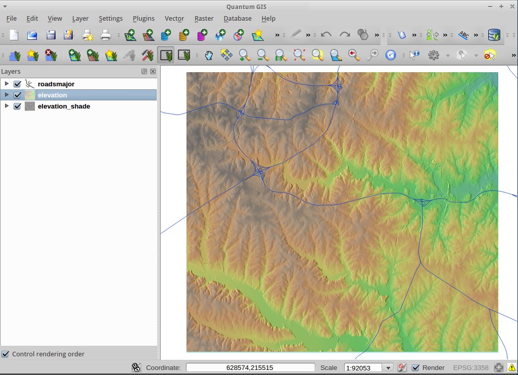
Add another GRASS raster layer, this time the elevation.10m map from the PERMANENT mapset.
To add a vector map, choose Plugins ‣ GRASS ‣ Add GRASS vector layer.
The plugin also gives you access to many of the powerful GRASS analysis modules and visualization tools:
A core plugin for QGIS which opens the door to a large family of processing tools is the Processing Toolbox (formerly named the SEXTANTE Toolbox). It acts as a standardized wrapper around a number of other sets to tools.
Open the LX Terminal Emulator from the main Accessories menu.
Cut and paste the following commands into the Terminal window to create a working copy of the OSM data in the home directory:
cp data/osm/feature_city_CBD.osm.bz2 .
bzip2 -d feature_city_CBD.osm.bz2
In QGIS, choose Project ‣ New. If you had the Processing Toolbox open you might want to close it.
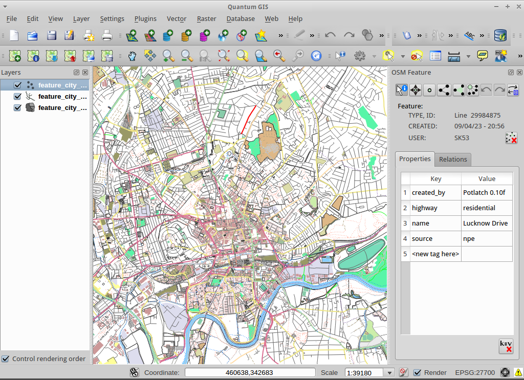
Choose Vector ‣ OpenStreetMap ‣ Import toplogy from XML.
Click on the ”...” button next to “Input XML file (.osm)” and select the feature_city_CBD.osm file you just copied into the home directory. The “Output SpatialLite DB file” name will be automatically set. Click Ok to convert the dataset to SpatiaLite format and create a connection to the SpatialLite DB within QGIS.
Next we need to extract points, lines, and areas, then add topology to each of these three new layers. To do this we need to run the tool three times. Select Vector ‣ OpenStreetMap ‣ Export toplogy to SpatiaLite and use the ”...” button to select the newly created feature_city_CBD.osm.db file. The Output layer name will be automatically filled in for you depending on the Export type selected. Click the Load from DB button to load in the available tags. For the “points” layer tick the amentity box; for the “polylines” layer tick the highway layer; and for the “polygon” layer select the building layer. You may wish to change the Output layer name to reflect the feature tags that you’ve selected. When you are ready, press Ok to load in the layer. You will need to again press the Load from DB button after changing the export type from points to polylines, and polylines to polygons.
Once topology is loaded, you can also refine the SpatiaLite layer by querying just certain features from within it. Select Layer ‣ Add SpatiaLite Layer... from the menu and from the Databases list select feature_city_CBD@... and then click on Connect. Double click on the feature_city_cbd_polylines table and then double click on “highway” to start building your SQL query. Then click on the = button, then the All button, and double click on motorway from the Values list. Click the Test button to verify the result, and finally click on Ok. Back in the Add SpatiaLite Table window click Add to restrict the rendering to just major highways. You can repeat this process with new layers to render different road types with different widths and styles.
You can now explore this rich dataset. Use the i information cursor button in the QGIS toolbar to query individal map features.
より進んだ QGIS のチュートリアルを OSGeo-Live QGIS tutorials に集めてあります。
QGIS について詳細の開始ページは QGIS ホームページの Documentation page になります。
A Gentle Introduction to GIS [1] eBook と QGIS User Guide [2] は OSGeo-Live のディスクに含まれています。