
R Quickstart
R is a free software environment for statistical computing and graphics.
This Quick Start describes how to:
use R for simple arithmetic
load some data from a shapefile and map it
do a coordinate transformation
plot some data points on a map
Start R
R is essentially a command-line program, although graphical user interfaces are available. You type a line of code at the prompt, press return, and the R interpreter evaluates it and prints the result.
Tip
Don’t fear the command line - it is a source of great power. Using the up and down arrows to recall commands so you can edit mistakes. Hit CTRL-C if get stuck and you should get the prompt back.
Choose . A terminal window opens running R.
You can start with simple arithmetic.
> 3*2
[1] 6

> 1 + 2 * 3 / 4
[1] 2.5

> sqrt(2)
[1] 1.414214

> pi * exp(-1)
[1] 1.155727
A full range of arithmetic, trigonometric, and statistical functions are built-in, and thousands more are available from packages in the CRAN archive.
The main prompt in R is >, but there is also the continuation prompt +, which
appears if R expects more input to make a valid expression. You’ll see this if you
forget a closing bracket or parenthesis.
> sqrt(
+ 2
+ )
[1] 1.414214
Building data
You might be wondering what the mysterious ‘one’ in square brackets is doing in the output. This is telling you that the result is one number. R can store things in one-dimensional vectors, two-dimensional matrices, and multi-dimensional arrays. There are many functions that can generate these things. Here’s a simple sequence:
> seq(1, 5, len=10)
[1] 1.000000 1.444444 1.888889 2.333333 2.777778 3.222222 3.666667 4.111111
[9] 4.555556 5.000000
Now you can see that the [9] is telling us that 4.555 is the ninth
value in the vector.
If you construct a matrix you get row and column labels:
> m = matrix(1:12, 3, 4)
> m
     [,1] [,2] [,3] [,4]
[1,]    1    4    7   10
[2,]    2    5    8   11
[3,]    3    6    9   12
Elements of matrices can be extracted using square brackets, with row and column indices separated by commas. Leave an index blank to get a whole row as a vector. Use a vector index to get multiple rows or columns as a smaller matrix:
> m[2,4]
[1] 11

> m[2,]
[1]  2  5  8 11

> m[,3:4]
     [,1] [,2]
[1,]    7   10
[2,]    8   11
[3,]    9   12
Data frames are data structures that mirror the kind of structure found in an RDBMS such as Postgres or MySQL. Each row can be thought of as a record, with columns being like fields in a database. As in a database, each field must be of the same type for each record.
In many ways they work like matrices, but you can also get and set the columns by name using $-notation:
> d = data.frame(x=1:10, y=1:10, z=runif(10)) # z is 10 random numbers
> d
        x  y          z
    1   1  1 0.44128080
    2   2  2 0.09394331
    3   3  3 0.51097462
    4   4  4 0.82683828
    5   5  5 0.21826740
    6   6  6 0.65600533
    7   7  7 0.59798278
    8   8  8 0.19003625
    9   9  9 0.24004866
    10 10 10 0.35972749

> d$z
 [1] 0.44128080 0.09394331 0.51097462 0.82683828 0.21826740 0.65600533
 [7] 0.59798278 0.19003625 0.24004866 0.35972749

> d$big = d$z > 0.6  # d$big is now a boolean true/false value
> d[1:5,]
  x y          z   big
1 1 1 0.44128080 FALSE
2 2 2 0.09394331 FALSE
3 3 3 0.51097462 FALSE
4 4 4 0.82683828  TRUE
5 5 5 0.21826740 FALSE

> d$name = letters[1:10] # create a new field of characters
> d[1:5,]
  x y          z   big name
  1 1 1 0.44128080 FALSE    a
  2 2 2 0.09394331 FALSE    b
  3 3 3 0.51097462 FALSE    c
  4 4 4 0.82683828  TRUE    d
  5 5 5 0.21826740 FALSE    e
Loading map data
There are many packages for spatial data manipulation and statistics. Some are included here, and some can be downloaded from CRAN.
Here we will load two shapefiles - the country boundaries and populated places from the Natural Earth data. We use two add-on packages to get the spatial functionality:
> library(sf) # Simple Features manipulation Library
> library(ggplot2) # Plotting library
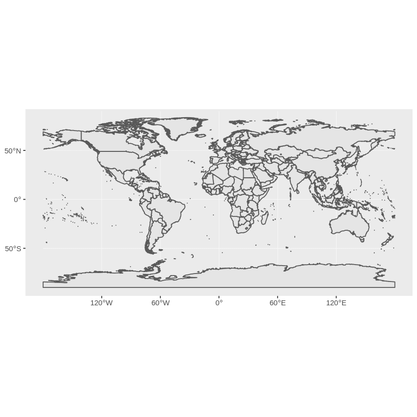
> countries <- st_read(dsn = "~/data/natural_earth2/ne_10m_admin_0_countries.shp")
> places <- st_read(dsn = "~/data/natural_earth2/ne_10m_populated_places.shp")
> ggplot(countries) + geom_sf()
This gives us a simple map of the world:
When an OGR dataset is read into R in this way we get back an object that
behaves in many ways like a data frame. We can use the admin
field to subset the world data and just get the UK:
> uk <- countries[countries$admin == 'United Kingdom',]
> ggplot(uk) + geom_sf()
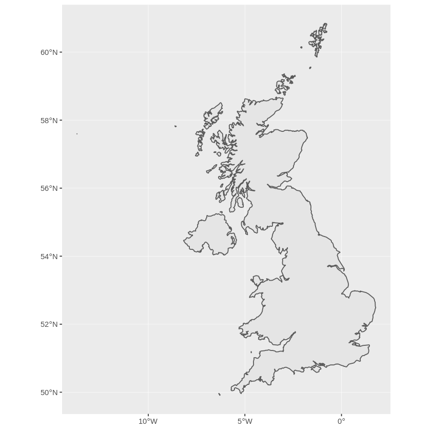
This looks a bit squashed to anyone who lives here, since we are more familiar with a coordinate system centred at our latitude. Currently the object doesn’t have a coordinate system assigned to it.
We need to assign a CRS to the object before we can transform it with the sf::st_transform function from the sf package. We transform to EPSG:27700 which is the Ordnance Survey of Great Britain grid system:
> ukos <- st_transform(uk,27700)
> ggplot(ukos) + geom_sf()

This plots the base map of the transformed data. Now we want to add some points from the populated place data set. Again we subset the points we want and transform them to Ordnance Survey Grid Reference coordinates:
> ukpop <- places[places$SOV0NAME == 'United Kingdom',]
> ukpop <- st_transform(ukpop,27700)
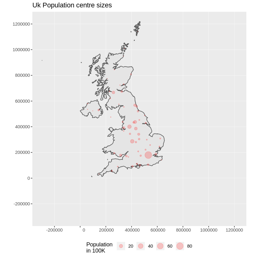
We add these points to the base map, scaling their size by scaled square root of the population (because that makes a symbol with area proportional to population), set the colour to red and the plotting character to a solid blob:
> ggplot() +
>   geom_sf(data = ukos) +                                                          # add UK shape to the map
>   geom_sf(data = ukpop,                                                           # add the Populated places
>           aes(size = ukpop$POP_MAX/100000),                       # fix size of points (by area)
>           colour = 'red', alpha = 1/5) +                          # set points colour and transparency
>   coord_sf(crs = 27700, datum= sf::st_crs(27700),         # set a bounding box
>            xlim = st_bbox(ukos[c(1,3)]),                          # for the map
>            ylim = st_bbox(ukos[c(2,4)])
>           ) +
>   ggtitle('Uk Population centre sizes') +                         # set the map title
>       theme(legend.position = 'bottom') +                         # Legend position
>           scale_size_area(name = 'Population \nin 100K')  # 0 value means 0 area + legend title
and our final image appears:
Tip
To quit R, type q() and hit return. R will ask you if you want to save your workspace as an R data image file. When you start R again from a directory with a .RData file it will restore all its data from there.
Vignettes
In the past, the documentation for R packages tended to be tersely-written help pages
for each function. Now package authors are encouraged to write a ‘vignette’ as a friendly
introduction to the package. If you run the vignette() function with no arguments
you will get the list of those vignettes on your system. Try vignette("sf1") for a
slightly technical introduction to the R spatial package.
What next?
For general information about R, try the official Introduction to R or any of the documentation from the main R Project page.
For more information on spatial aspects of R, the best place to start is probably the R Spatial Task View
You might also want to check out the R-Spatial and RSpatial pages.