
Live DVDでGRASSを起動するには, Geospatial ‣ デスクトップ GIS メニューをクリックして下さい. “GRASSへようこそ” と書かれた起動画面にて, ロケーションにSpearfishデータセット, マップセットに “user1” を選択し, [Start Grass] をクリックしてください.
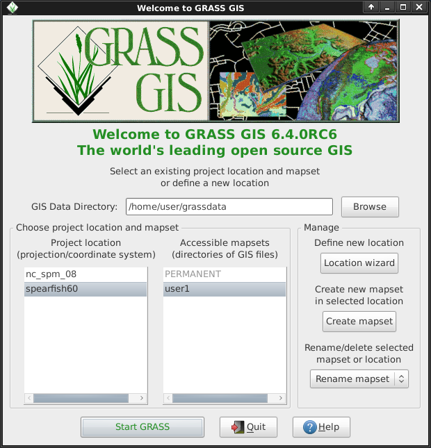
このようにすると, wxPythonで書かれた新しいGUI のGRASSが起動します.
Tip
画面の小さい (800 x 600 解像度) ネットブックの場合は起動画面がくずれて
[Start GRASS] ボタンがロケーションやマップセットのリストに隠れてしまうかもしれません. その場合はウィンドウの端をドラッグしてウィンドウを大きくしてください. ウィンドウを画面の上にずらす必要があるかもしれません (Altキーを押しながら左クリックでドラッグするとウィンドウを動かせます).
ディスクにはノースカロライナ (nc_basic_spm) の簡易版データも収録されています, このクィックチュートリアルは Spearfish データセット用に作成されているので使用データごとに読み替えて下さい. また, 使用するデータに関わらず作業には PERMANENT マップセットではなく user マップセットの使用をお勧めします.
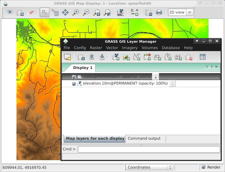
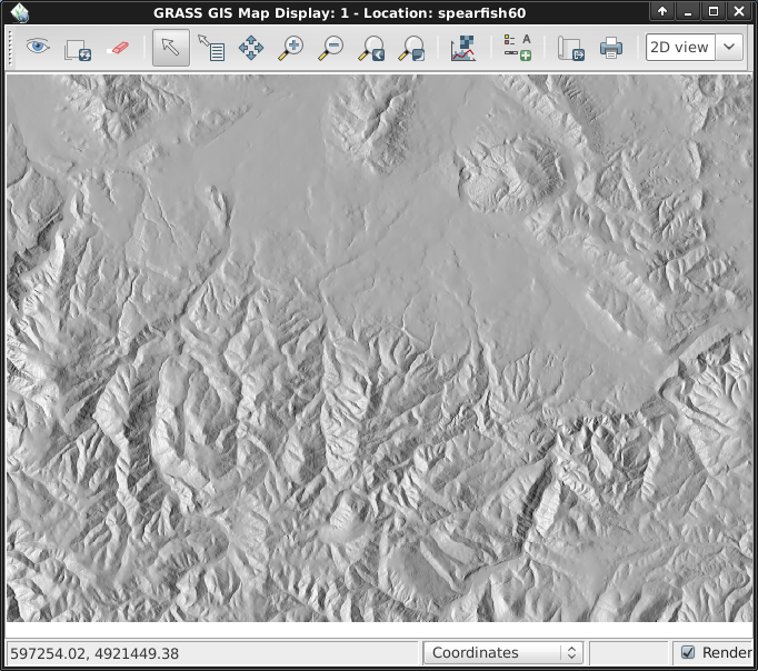
PERMANENT マップセットから “elevation.10m” といったラスターレイヤーを加えます. GIS レイヤマネージャ ウィンドウにて “+” 記号のついたツールバーボタンをクリックして下さい. そして “表示するマップ” リストからマップ名を選択して, Ok をクリックして下さい.
同様に “roads” ベクターレイヤーも PERMANENT マップセットから “+” 記号のついたV字に見える線のツールバーボタンをクリックして追加して下さい.
必要なら, ラスターマップ名を右クリックして “選択したマップのズーム” を選択して下さい.
マップが表示されていますよね.
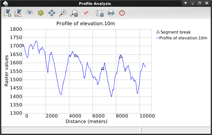
GIS レイヤマネージャ ウィンドウに戻って`elevation.10m`ラスターを選択するために名前をクリックして下さい. マップディスプレイ ウィンドウで マップ表示 ツールバーのズームボタンの右にある線と縞目模様のあるアイコンを見て下さい. Profile surface map をクリックして選択して下さい. @PERMANENT マップセットは自動的に検索されて, ファイル名で絞り込むことができます. もし自動的にリストに表示がされない場合は, 再び elevation.10m マップをラスターレイヤーとして選択して Ok をクリックして下さい. 左から2番目のボタンをクリックして, Map Display キャンバスのの複数点をクリックすることでプロファイルを取ることができます. 何点かクリックしたのちプロファイルウィンドウの目玉ボタンをクリックするとプロファイルを表示することができます. 終了するには右端にあるスイッチボタンをクリックして下さい.
Now let’s create a new map. First set the computational region to the default bounds with Settings ‣ Region ‣ Set region, ticking “Set from default region”, and clicking [Run]. Next select Raster ‣ Generate surfaces ‣ Fractal surface from the menu (it’s near the bottom); give your new map a name; and adjust any options you like in the “Optional” tab (the defaults are fine); and click [Run]. You can then [Close] the r.surf.fractal module’s dialog window.
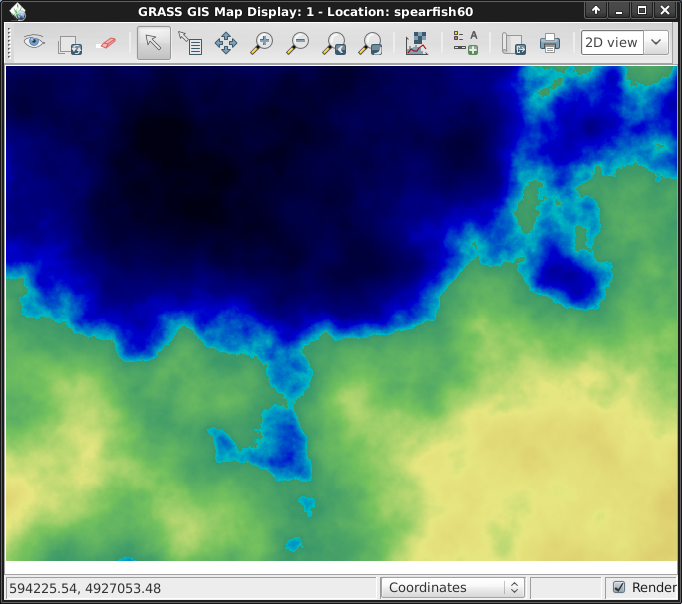
新しいラスターマップが標高マップとともにレイヤーリストないしは “user1” マップセットに加わっているとのが見えると思います. elevation.10m レイヤの表示チェックボックスをオフにすることで表示を制御することができます. 自動的に表示されない場合は目玉をクリックすると表示がされるようになります. The colors might not be as you’d like so let’s change them. With the fractal DEM selected in the layer list, in the Raster menu select Manage colors ‣ Color tables. In the “Colors” tab click on the pull-down list for the “Type of color table” option, and pick one from the list. “srtm” is a nice choice. Once done click the [Run] button and close the r.colors dialog window. The colors should then update automatically.
Next we’ll create a shaded relief map of the elevation layer we saw earlier. Start by verifying that the computational region is set match the raster map of interest, “elevation.10m” in the PERMANENT mapset. To do this, make sure it is loaded into the layer list of the main GIS Layer Manager window, right click on its name and select “Set computation region from selected map(s)”. You will notice the Layer Manage tab will switch to a text console to display the new settings. Click on the “Map layers” tab at the bottom to get back to the layer list.
In the Raster menu select Terrain analysis ‣ Shaded relief (Terrain analysis is about half way down), and the module control dialog will appear. With the elevation map name selected as the input map click [Run]. Now add the new elevation.shade @user1 map into your layer list as you did for the elevation.10m map earlier, and un-tick the other raster layers.
Once again select the elevation.10m @PERMANENT map. If you changed the region since the last step, again right click on the layer name and click on Set computational region from selected map(s) from the context menu.
Note
The wxGUI map display’s view and zoom is independent and does not affect processing calculations. Check the computational region at any time with Settings ‣ Region ‣ Display Region; this is of fundamental importance to any raster grid operations. Raster maps of differing bounds and resolution will be resampled to the current computational region on-the-fly.
Next, in the Raster menu choose Hydrologic modeling ‣ Watershed analysis. This will open the r.watershed module. Select the elevation.10m layer as your input map, in the ‘Input options’ tab set the minimum size of the exterior watershed basin threshold to 10000 cells, then in the ‘Output options’ tab enter “elev.basins” for the watershed basin option and “elev.streams” for the stream segments option just below it. Then click [Run].
Back in the GIS Layer Manager window check that those two new raster maps are in the layer list and make sure that the basins map is ticked for display in the box to the left of the layer name. You might untick the streams map for now. Next, right click on the “elev.basins” raster map layer name and select “Change opacity level”. Set it to about 50% which will re-render the Map Display. Drag a map layer (such as the earlier shaded relief map) to lower down in the layer list if you wish for it to be drawn behind the watershed basins map layer, and make sure to tick its visibility box to view it as a backdrop.
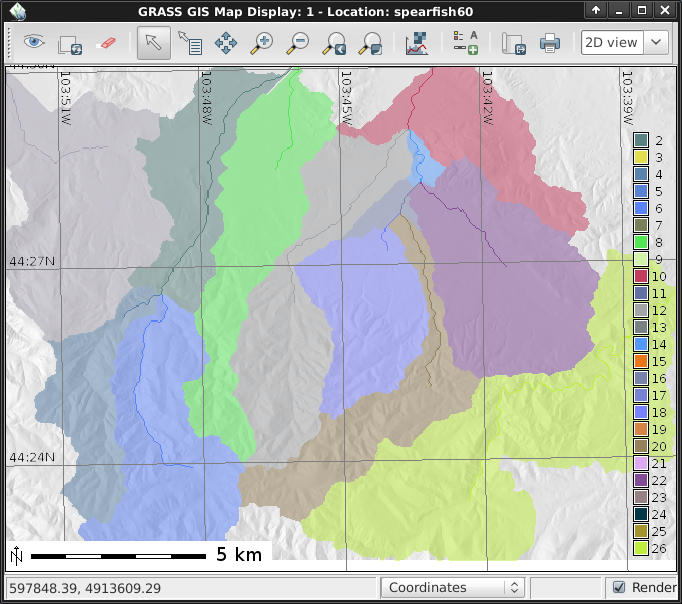
In the GIS Layer Manager window click on the second button in from the right on the top row and Add a grid layer. For size of grid put 0:03 for 0 degrees and 3 minutes (format is D:M:S), then in the “Optional” tab tick Draw geographic grid and press Ok and re-render. You may need to drag the new grid layer higher up on the layer list to see it.
To add a scalebar go to the Map Display window and press the “Add map elements” button to the right of where you selected the Profile tool earlier and select “Add scalebar and north arrow” then click Ok. A scalebar will appear in the top left of the map canvas. Drag it down to the bottom left. From the same toolbar menu select “Add legend” and in the instructions window click the Set Options button to set the raster map name to create the legend for. If you pick the elev.basins map you will want to set the Thinning factor to 10 in the Advanced tab, and the Placement position to 5,95,2,5 in the Optional tab. After you are done click Ok and Ok again. Drag your new legend over to the right side of the map canvas.
Now you may be thinking to yourself that these fonts are a bit bare. That’s easily fixed in the GIS Layer Manager menus open Settings ‣ Preferences and in the Map Display tab click the [Set font] button, choose one (for example DroidSans), and then [Apply] in the Preferences window. You will have to do a full re-render to see the change so click on the re-render button next to the eyeball in the Map Display window. The fonts will now be much prettier.
The above tasks have only covered a few raster modules. Don’t let this give you the idea that GRASS is just for raster maps – the vector engine and modules are every bit as full-featured as the raster ones. GRASS maintains a fully topological vector engine which allows all sorts of very powerful analyses.
Continuing with the watershed basins created above, next we’ll convert them into vector polygons. In the Raster menu select Map type conversions ‣ Raster to vector. In the r.to.vect dialog that opens make sure that elev.basins @user1 is selected for the input map, give a name for the output map like basins_areas (vector map names must be SQL compliant), and change feature type to area. In the Attributes tab tick the box to use raster values as category numbers, since these will match the values in our stream segment raster map created earlier. Then click on [Run]. Once the new vector map is displayed, you might right click on it in the Layer Manager list and change its opacity level. Also if you right click on the basins_areas vector map in the Layer List you can turn off rendering of area centroids by going into Properties and un-ticking it in the Selection tab.
Next we’ll add some attributes to those new areas, containing the average elevation in each basin. In the Vector menu select Update attributes ‣ Update area attributes from raster to launch the v.rast.stats module. Use basin_areas as the vector polygon map, the elevation.10m raster to calculate the statistics from, make the column prefix ele, and click [Run] then close the dialog when it is finished. You can query the values in the Map Display window using the fifth icon from the left and after verifying that the vector-areas map is selected in the Layer List, clicking on a vector area in the map canvas.
You can colorize the areas based on the average elevation values using the v.colors module. In the Vector menu select Manage colors ‣ Color tables. Select basin_areas for the input vector map, the ele_mean attribute column for the column containing the numeric range, and in the Colors tab have it copy the colors from the elevation.10m raster map. After running that right-click on the basin_areas map in the Layer List and select Properties. In the Colors tab tick the box for getting colors from the map table column. Once you click [Apply] you should see the colors change in the Map Display window.
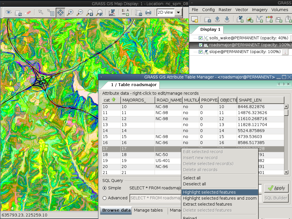
Now let’s look at the attribute table and SQL builder in more detail. In the Layer Manager click the table icon, it’s second from the left on the bottom row. This will open a view of the attached database table. For now we’ll just do a Simple database query to find watershed basins without a lot of variation in them. Where it says SELECT * FROM basin_areas WHERE pick ele_stddev from the pull down list for the standard deviation statistic, then in the text box to its right enter < 50 and click [Apply]. You’ll notice the number of loaded records in the information bar along the bottom of the window has shrunk, and that all of the rows with large values for std. dev. are now gone from the displayed table. Right-click on the table data and choose Select all. Again right-click on the table data and this time choose Highlight selected features. You should see e.g. alluvial flood basins and mesas show up in the Map Display.
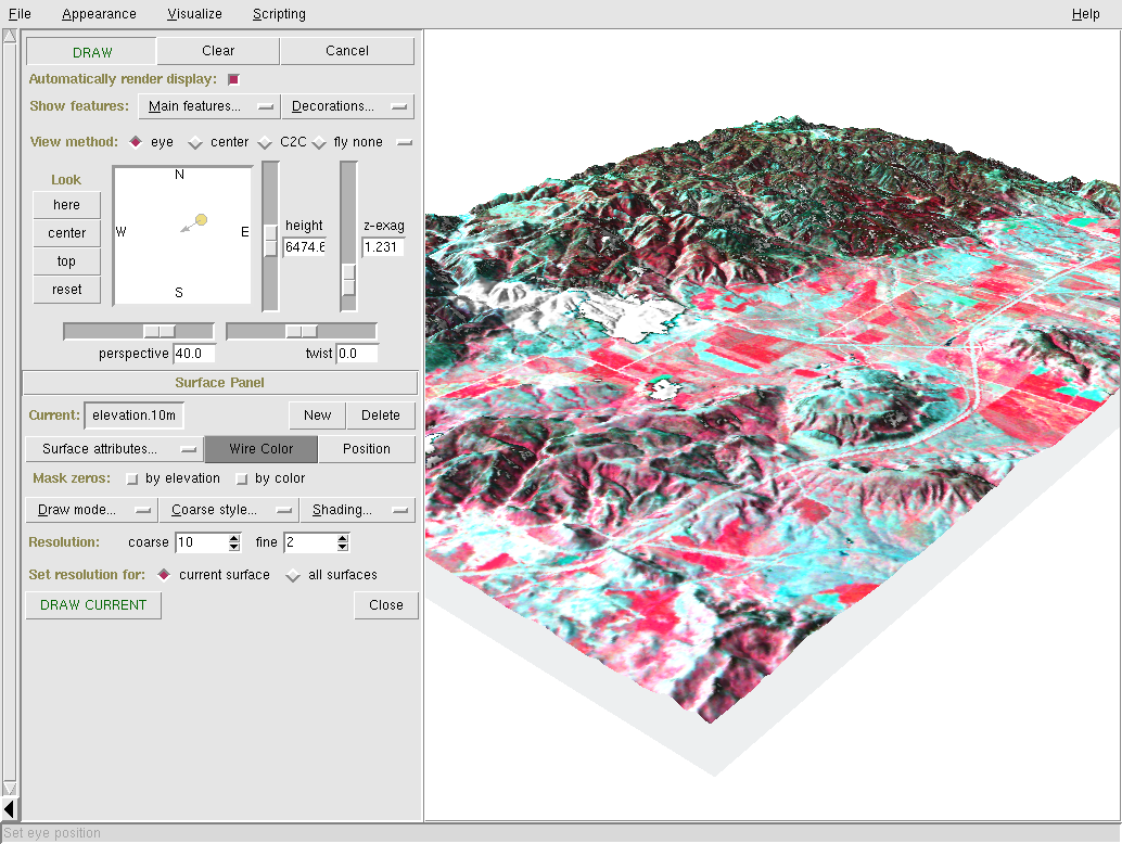
Start the 3D visualization suite from the File ‣ NVIZ menu item. Select the elevation.10m map as the raster elevation and click [Run]. Once the 3D display interface loads, maximize the window. Next select Visualize ‣ Raster Surfaces from the top menu, and set the fine resolution to “1”, then move the positioning puck and height slider around to get different views.
To drape satellite or aerial imagery over the top of the DEM, in the Raster Surfaces controls click on the Surface Attributes drop down menu and select “color”. Select “New Map” to pick the overlay image; “spot.image” in the PERMANENT mapset is a good choice. Finally, click “Accept” and then once back at the main window click on the “Draw” button in the top-left, just under the File menu.
While not covered here, you may like to experiment with the new Cartographic Composer and object-oriented Graphical Modeling Tool; you’ll find icons to launch them on the lower row of icons in the Layer Manager window. Further details can be found in the wxGUI help pages.
The new GUI is written in Python, and if you’re a fan of Python programming there are a number of great tools available to you. In the bottom of the Layer Manager window click on the Python shell tab and type help(grass.core) to see a listing of the many functions available in the core GIS python library. Besides the core GIS functions there is also array (NumPy), db (database), raster, and vector libraries available. For advanced use Pythons CTypes is supported allowing the Python programmer direct access to GRASS’s extensive C libraries.
When finished, exit the GRASS GUI with File ‣ Exit GUI. Before you close the GRASS terminal session as well, try a GRASS module by typing “g.manual --help” which will give you a list of module options. The GRASS command line is where the true power of the GIS comes into its own. GRASS is designed to allow all commands to be tied together in scripts for large bulk processing jobs. Popular scripting languages are Bourne Shell and Python, and many neat tricks to help make scripting easier are included for both. With these tools you can make a new GRASS module with only about 5 minutes of coding, complete with powerful parser, GUI, and help page template.
“g.manual -i” will launch a web browser with the module help pages. When you are done close the browser and type “exit” at the GRASS terminal prompt to leave the GIS environment.