

Note
This project is only included on the OSGeoLive virtual machine disk (VMDK)
actinia Quickstart
Actinia is an open source REST API for scalable, distributed, high performance processing of geographical data that uses mainly GRASS GIS for computational tasks. Actinia provides a REST API to process satellite images, time series of satellite images, raster and vector data.
Contents
Actinia can be used in different ways:
curl or similar command line tools
through Jupyter notebooks
the Python interface
the Postman or RESTman extension for browsers
open a GRASS GIS session and use the ace (actinia command execution) tool
other interfaces to REST API
In this quickstart, we make use of GRASS GIS to conveniently launch commands from the session to the actinia server (which itself uses GRASS GIS). The idea is to rapidly develop a workflow locally on small data sets to then execute it on the server.
Using actinia with a Jupyter notebook
Numerous Jupyter notebooks for actinia are available from https://github.com/actinia-org/actinia-jupyter
Introduction to ace - actinia command execution
The ace tool (details)
allows the execution of a single GRASS GIS command or a
list of GRASS GIS commands on an actinia REST service
(https://actinia.mundialis.de/). In addition it provides job management,
the ability to list locations, mapsets and map layer the user has access
to as well as the creation and deletion of mapsets.
Th ace tool must be executed in an active GRASS GIS session. It is
installed with g.extension extension=ace url=https://github.com/actinia-org/ace.
All commands will be executed per default in an ephemeral database. Hence, generated output must be exported using augmented GRASS commands.
The option mapset=MAPSET_NAME allows the execution of commands in
the persistent user database. It can be used with
location=LOCATION_NAME option.
Setup your environment
Be sure to run the following commands in a GRASS GIS session.
The user must setup the following environmental variables to specify the actinia server and credentials:
# set credentials and REST server URL
export ACTINIA_USER='demouser'
export ACTINIA_PASSWORD='gu3st!pa55w0rd'
export ACTINIA_URL='https://actinia.mundialis.de/latest'
Access sample data
Selected datasets are available to the demo user. To list the locations you have access to, run
ace -l
['latlong_wgs84', 'ECAD', 'nc_spm_08']
The following command lists mapsets of current location in the active GRASS GIS session (nc_spm_08):
# running ace in the "nc_spm_08" location
# (the current location name is propagated to the server):
ace location="nc_spm_08" -m
['PERMANENT', 'landsat', 'modis_lst']
Access data from external sources
GRASS GIS commands can be augmented with actinia specific extensions.
The @ operator can be specified for an input parameter to import a
web located resource and to specify the export of an output parameter.
Importantly, the name of the local location and mapset must correspond to that on the actinia REST server.
Currently available datasets are (organized by projections):
North Carolina sample dataset (NC State-Plane metric CRS, EPSG: 3358):
base cartography (
nc_spm_08/PERMANENT; source: https://grassbook.org/datasets/datasets-3rd-edition/)Landsat subscenes (
nc_spm_08/landsat; source: https://grass.osgeo.org/download/data/)
Latitude-Longitude location (LatLong WGS84, EPSG:4326):
empty (
latlong_wgs84/PERMANENT/)16-days NDVI, MOD13C1, V006, CMG 0.05 deg res. (
latlong_wgs84/modis_ndvi_global/; source: https://lpdaac.usgs.gov/products/mod13c1v006/)LST growing degree days asia 2017 (
latlong_wgs84/asia_gdd_2017/; source: https://www.mundialis.de/en/temperature-data/)LST tropical days asia 2017 (
latlong_wgs84/asia_tropical_2017/)LST temperature daily asia 2017, including min, max and avg (
latlong_wgs84/asia_lst_daily_2017/)
Europe (EU LAEA CRS, EPSG:3035):
EU DEM 25m V1.1 (
eu_laea/PERMANENT/; source: https://land.copernicus.eu/imagery-in-situ/eu-dem)CORINE Landcover 2012, g100_clc12_V18_5 (
eu_laea/corine_2012/; source: https://land.copernicus.eu/pan-european/corine-land-cover/clc-2012)
World Mollweide (EPSG 54009):
GHS_POP_GPW42015_GLOBE_R2015A_54009_250_v1_0 (
world_mollweide/pop_jrc; source: https://ghsl.jrc.ec.europa.eu/ghs_pop.php)
Inspect the REST call prior to submission
To generate the actinia process chain JSON request simply add the
-d (dry-run) flag:
ace location="nc_spm_08" grass_command="r.slope.aspect elevation=elevation slope=myslope" -d
Display a map - map rendering
It is very easy (and fast) to render a map:
# check amount of pixels, just FYI
ace location="latlong_wgs84" grass_command="r.info globcover@globcover"
# render the map ... 7 billion pixels
ace location="latlong_wgs84" render_raster="globcover@globcover"
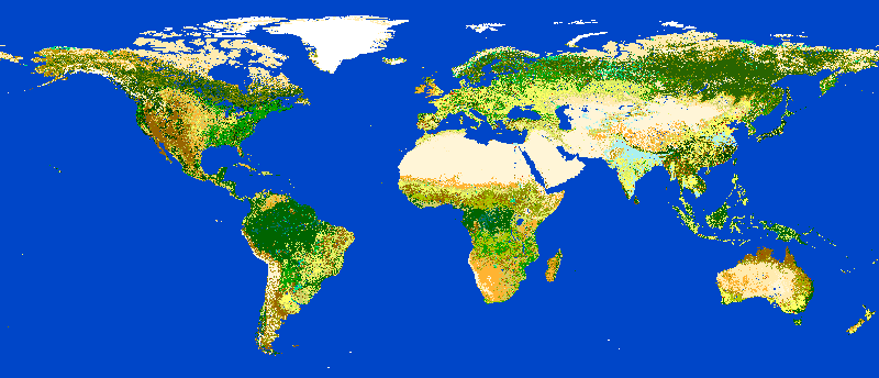
ESA Globcover map shown by actinia
Ephemeral processing is the default processing approach of actinia. Commands are executed in an ephemeral mapset which will be removed after processing. You can export the output of GRASS GIS modules to store the computational result for download and further analysis. The following export formats are currently supported:
raster:
COG,GTiffvector:
GPKG,GML,GeoJSON,ESRI_Shapefiletable:
CSV,TXT
Script examples
Example 1: computing slope and aspect and univariate statistics from an elevation model
The following commands (to be stored in a script and executed with
ace) will import a raster layer from an internet source as raster
map elev, sets the computational region to the map and computes the
slope. Additional information about the raster layer are requested with
r.info.
Store the following script as text file ace_dtm_statistics.sh:
# grass ~/grassdata/nc_spm_08/user1/
# Import the web resource and set the region to the imported map
g.region raster=elev@https://storage.googleapis.com/graas-geodata/elev_ned_30m.tif -ap
# Compute univariate statistics
r.univar map=elev
r.info elev
# Compute the slope of the imported map and mark it for export as a COG file (Cloud Optimized GeoTIFF)
r.slope.aspect elevation=elev slope=slope_elev+COG
r.info slope_elev
Save the script in the text file to /tmp/ace_dtm_statistics.sh and
run the saved script as
ace --location nc_spm_08 --script ace_dtm_statistics.sh
The results (messages, statistics, files) are provided as REST resources.
To generate the actinia process chain JSON request simply add the
-d (dry-run) flag:
ace -d location="nc_spm_08" script="/tmp/ace_dtm_statistics.sh"
The output should look like this:
{
  "version": "1",
  "list": [
    {
      "module": "g.region",
      "id": "g.region_1804289383",
      "flags": "pa",
      "inputs": [
        {
          "import_descr": {
            "source": "https://storage.googleapis.com/graas-geodata/elev_ned_30m.tif",
            "type": "raster"
          },
          "param": "raster",
          "value": "elev"
        }
      ]
    },
    {
      "module": "r.univar",
      "id": "r.univar_1804289383",
      "inputs": [
        {
          "param": "map",
          "value": "elev"
        },
        {
          "param": "percentile",
          "value": "90"
        },
        {
          "param": "separator",
          "value": "pipe"
        }
      ]
    },
    {
      "module": "r.info",
      "id": "r.info_1804289383",
      "inputs": [
        {
          "param": "map",
          "value": "elev"
        }
      ]
    },
    {
      "module": "r.slope.aspect",
      "id": "r.slope.aspect_1804289383",
      "inputs": [
        {
          "param": "elevation",
          "value": "elev"
        },
        {
          "param": "format",
          "value": "degrees"
        },
        {
          "param": "precision",
          "value": "FCELL"
        },
        {
          "param": "zscale",
          "value": "1.0"
        },
        {
          "param": "min_slope",
          "value": "0.0"
        }
      ],
      "outputs": [
        {
          "export": {
            "format": "COG",
            "type": "raster"
          },
          "param": "slope",
          "value": "slope_elev"
        }
      ]
    },
    {
      "module": "r.info",
      "id": "r.info_1804289383",
      "inputs": [
        {
          "param": "map",
          "value": "slope_elev"
        }
      ]
    }
  ]
}
Example 2: Orthophoto image segmentation with export
Store the following script as text file /tmp/ace_segmentation.sh:
# grass ~/grassdata/nc_spm_08/user1/
# Import the web resource and set the region to the imported map
# we apply a importer trick for the import of multi-band GeoTIFFs:
# install with: g.extension importer url=https://github.com/actinia-org/importer
importer raster=ortho2010@https://apps.mundialis.de/workshops/osgeo_ireland2017/north_carolina/ortho2010_t792_subset_20cm.tif
# The importer has created three new raster maps, one for each band in the geotiff file
# stored them in an image group
r.info map=ortho2010.1
r.info map=ortho2010.2
r.info map=ortho2010.3
# Set the region and resolution
g.region raster=ortho2010.1 res=1 -p
# Note: the RGB bands are organized as a group
# export as a as COG file (Cloud Optimized GeoTIFF)
i.segment group=ortho2010 threshold=0.25 output=ortho2010_segment_25+COG goodness=ortho2010_seg_25_fit+COG
# Finally vectorize segments with r.to.vect and export as a GeoJSON file
r.to.vect input=ortho2010_segment_25 type=area output=ortho2010_segment_25+GeoJSON
Run the script saved in a text file as
ace location="nc_spm_08" script="/tmp/ace_segmentation.sh"
The results (messages, statistics, files) are provided as REST resources.
Examples for persistent processing
GRASS GIS commands can be executed in a user specific persistent
database. The user must create a mapset in an existing location. This
mapsets can be accessed via ace. All processing results of commands
run in this mapset, will be stored persistently. Be aware that the
processing will be performed in an ephemeral database that will be moved
to the persistent storage using the correct name after processing.
To create a new mapset in the nc_spm_08 location with the name test_mapset the following command must be executed
ace location="nc_spm_08" create_mapset="test_mapset"
Run the commands from the statistic script in the new persistent mapset
ace location="nc_spm_08" mapset="test_mapset" script="/path/to/ace_dtm_statistics.sh"
Show all raster maps that have been created with the script in test_mapset
ace location="nc_spm_08" mapset="test_mapset" grass_commmand="g.list type=raster mapset=test_mapset"
Show information about raster map elev and slope_elev
ace location="nc_spm_08" mapset="test_mapset" grass_command="r.info elev@test_mapset"
ace location="nc_spm_08" mapset="test_mapset" grass_command="r.info slope_elev@test_mapset"
Delete the test_mapset (always double check names when deleting)
ace location="nc_spm_08" delete_mapset="test_mapset"
If the active GRASS GIS session has identical location/mapset names, then an alias can be used to avoid the persistent option in each single command call:
alias acp="ace --persistent `g.mapset -p`"
We assume that in the active GRASS GIS session the current location is nc_spm_08 and the current mapset is test_mapset. Then the commands from above can be executed in the following way:
ace location="nc_spm_08" create_mapset="test_mapset"
acp location="nc_spm_08" script="/path/to/ace_dtm_statistics.sh"
acp location="nc_spm_08" grass_command="g.list type=raster mapset=test_mapset"
acp location="nc_spm_08" grass_command="r.info elev@test_mapset"
acp location="nc_spm_08" grass_command="r.info slope_elev@test_mapset"
Things to try
Install on OSGeoLive VM with Docker Compose
Requirements: docker and docker-compose (already available in OSGeoLive VM version)
To build and deploy actinia, run
git clone https://github.com/actinia-org/actinia-core.git
cd actinia_core
docker-compose -f docker/docker-compose.yml up
Now you have a running actinia instance locally! Check with
curl http://127.0.0.1:8088/api/v3/version
Create new locations
# (note: the "demouser" is not enabled for this)
#
# create new location
ace create_location="mylatlon 4326"
# create new mapset within location
ace location="mylatlon" create_mapset="user1"
Install GRASS GIS addons (extensions)
# (requires elevated user privileges)
#
# list existing addons, see also
# https://grass.osgeo.org/grass-stable/manuals/addons/
ace location="latlong_wgs84" grass_command="g.extension -l"

# install machine learning addon r.learn.ml2
ace location="latlong_wgs84" grass_command="g.extension extension=\"r.learn.ml2\""
What next?
Visit the actinia website at https://actinia.mundialis.de
actinia tutorial: https://neteler.gitlab.io/actinia-introduction
Further reading: Neteler, M., Gebbert, S., Tawalika, C., Bettge, A., Benelcadi, H., Löw, F., Adams, T, Paulsen, H. (2019). Actinia: cloud based geoprocessing. In Proc. of the 2019 conference on Big Data from Space (BiDS’2019) (pp. 41-44). EUR 29660 EN, Publications Office of the European Union 5, Luxembourg: P. Soille, S. Loekken, and S. Albani (Eds.). (DOI)